21. Hoja de Respuestas
21.1. Results For Añadiendo Tu Primera Capa
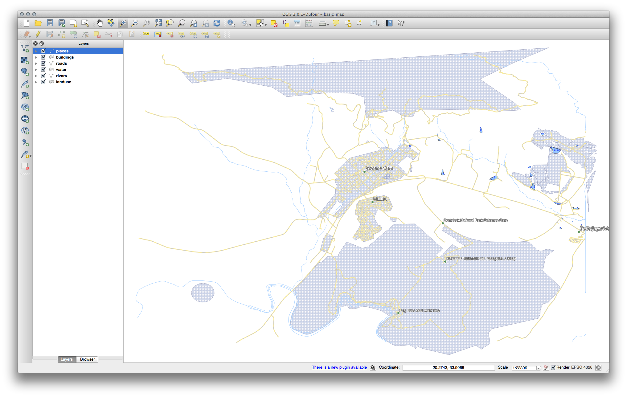
21.1.1.  Preparación
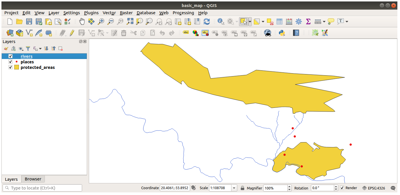
In the main area of the dialog you should see many shapes with different colors. Each shape belongs to a layer you can identify by its color in the left panel (your colors may be different from the ones below):
21.2. Results For Un resumen de la Interfaz
21.2.1. Resumen (Parte 1)
Refiérase a la imagen que muestra el diseño de la interfaz y comprobar que recuerdas los nombres y las funciones de los elementos de la pantalla.
21.2.2. Resumen (Parte 2)
Guardar como
Zoom a la capa
Invert selection
Renderizado on/off
Línea de medida
21.3. Results For Trabajando con Datos Vector
21.3.1. Attribute data
There should be 9 fields in the rivers layer:
Select the layer in the Layers panel.
Right-click and choose Open Attribute Table, or press the
 button on the Attributes Toolbar.
Count the number of columns.
Truco
A quicker approach could be to double-click the rivers layer, open the tab, where you will find a numbered list of the table’s fields.
Information about towns is available in the places layer. Open its attribute table as you did with the rivers layer: there are two features whose place attribute is set to
town: Swellendam and Buffeljagsrivier. You can add comment on other fields from these two records, if you like.
21.3.2. Data loading
Your map should have seven layers:
protected_areas
lugares
rivers
roads
landuse
buildings (taken from
training_data.gpkg) andwater (taken from
exercise_data/shapefile).
21.4. Results For Simbología
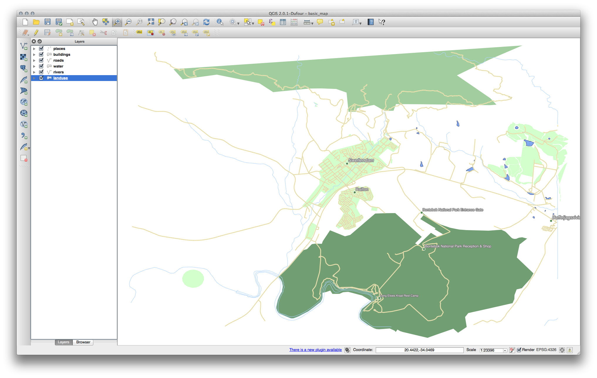
21.4.1. Colores
Comprueba que los colores están cambiando como esperas que cambien.
It is enough to select the water layer in the legend and then click on the
 Open the Layer Styling panel button. Change the color
to one that fits the water layer.
Open the Layer Styling panel button. Change the color
to one that fits the water layer.

Nota
If you want to work on only one layer at a time and don’t want the other layers to distract you, you can hide a layer by clicking in the checkbox next to its name in the layers list. If the box is blank, then the layer is hidden.
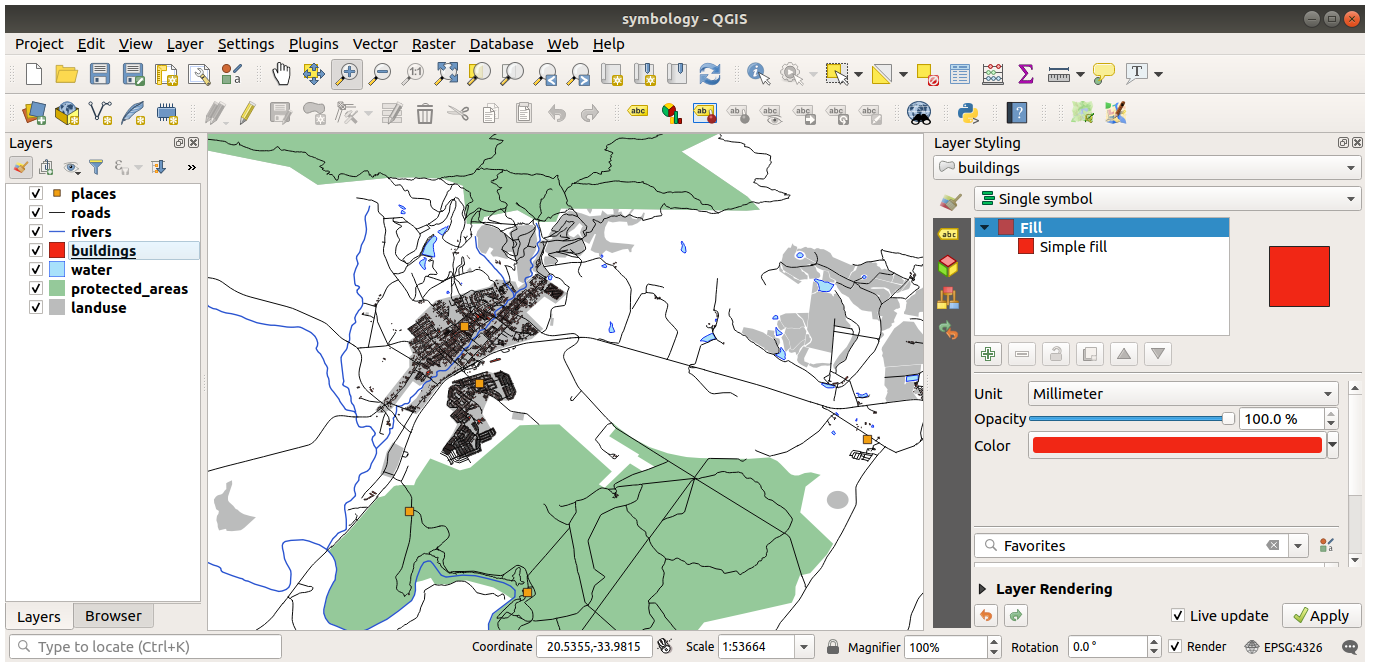
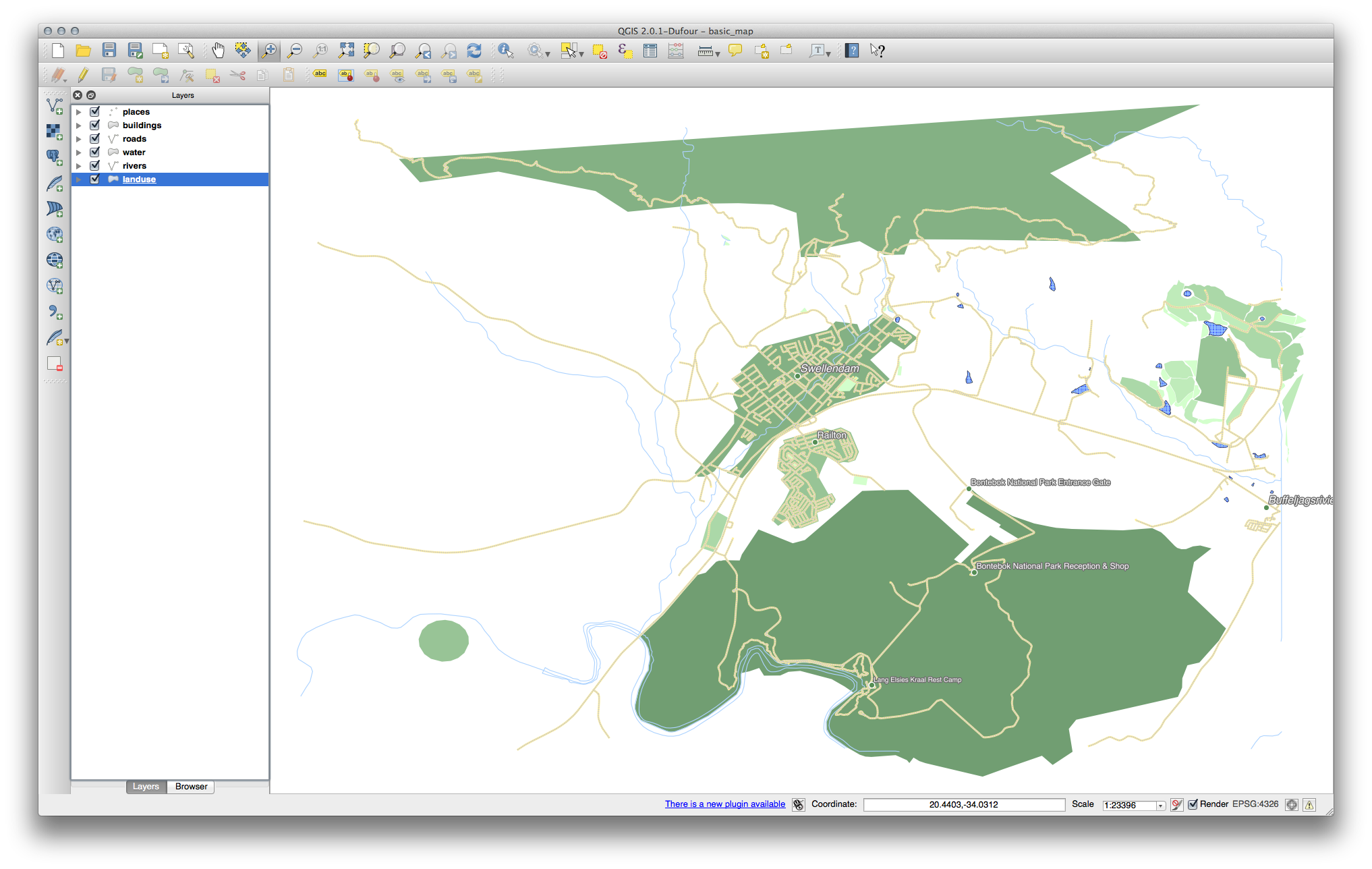
21.4.2. Estructura de símbolos
Ahora tu mapa debería aparecer así:

Si tu eres un usuario principiante, puede detenerse aquí.
Use el método anterior para cambiar los colores y estilos a todas las capas restantes.
Trata de usar colores naturales para los objetos. Por ejemplo, una carretera no debería ser roja o azul, pero si puede ser gris o negro.
Also feel free to experiment with different Fill style and Stroke style settings for the polygons.
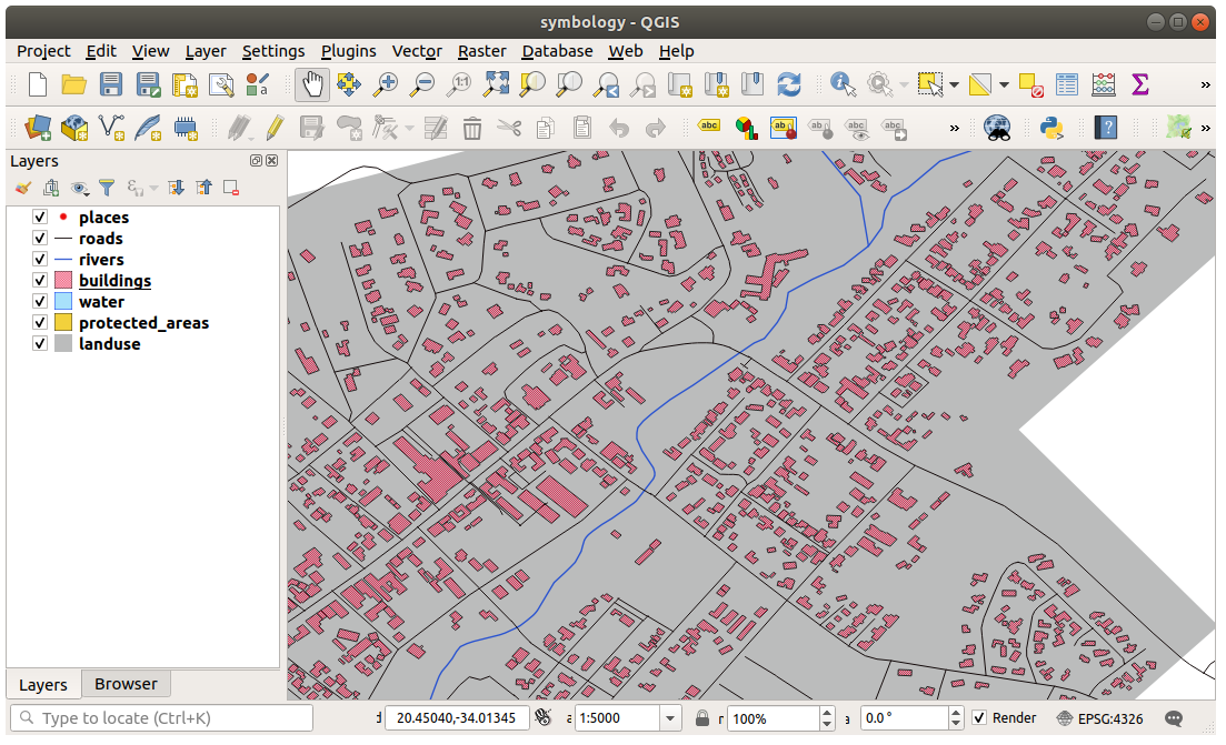
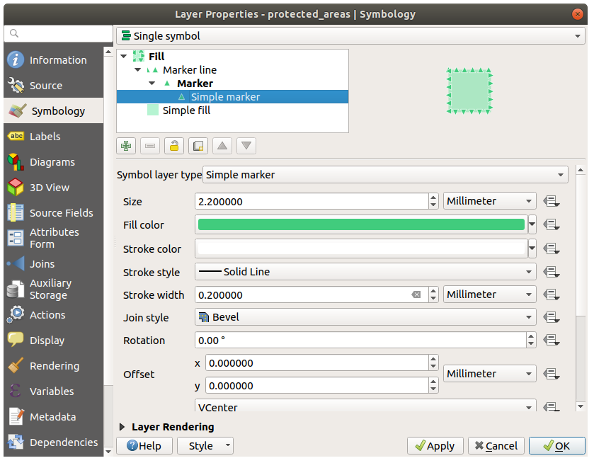
21.4.3.  Capas de símbolos
Personaliza tu construcciones capa como gustes, pero recuerda que tiene que ser fácil de contar las diferentes partes del mapa.
He aquí un ejemplo:
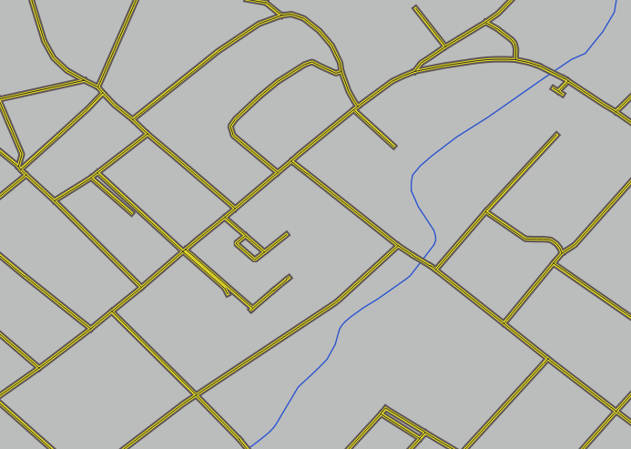
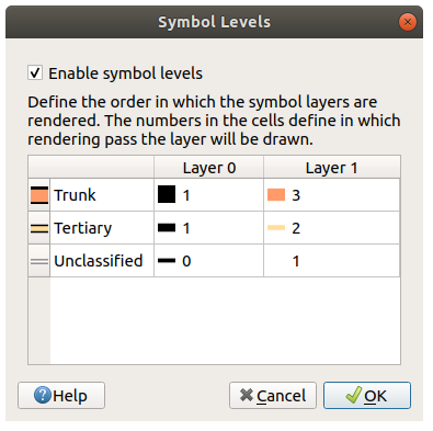
21.4.4. Niveles de símbolo
To make the required symbol, you need three symbol layers:

The lowest symbol layer is a broad, solid gray line. On top of it there is a slightly thinner solid yellow line and finally another thinner solid black line.
If your symbol layers resemble the above but you’re not getting the result you want:
Check that your symbol levels look something like this:

Ahora tu mapa debería tener este aspecto:
21.4.5.  Niveles de símbolo
Ajustar tus niveles de símbolo a estos valores:
Probar con diferentes valores para dar diferentes resultados.
Abrir de nuevo su mapa original antes de continuar con el siguiente ejercicio.
21.5. Outline Markers
Here are examples of the symbol structure:

21.5.1. Geometry generator symbology
Click on the
 button to add another Symbol level.
Move the new symbol at the bottom of the list clicking the
 button.
Choose a good color to fill the water polygons.
Click on Marker of the Geometry generator symbology and change the circle with another shape as your wish.
Try experimenting other options to get more useful results.
21.6. Results For Atributo de dato
21.6.1. * Atributo de dato*
The name field is the most useful to show as labels. This is because all its
values are unique for every object and are very unlikely to contain NULL
values. If your data contains some NULL values, do not worry as long as most
of your places have names.
21.7. Results For Labels
21.7.1. Personalizarción de Etiqueta (Parte 1)
Your map should now show the marker points and the labels should be offset by 2mm. The style of the markers and labels should allow both to be clearly visible on the map:

21.7.2. Personalizarción de Etiqueta (Parte 2)
Una posible solución tiene este producto final:
Para llegar a este resultado:
Use a font size of
10Use an around point placement distance of
1.5 mmUse a marker size of
3.0 mmIn addition, this example uses the Wrap on character option:
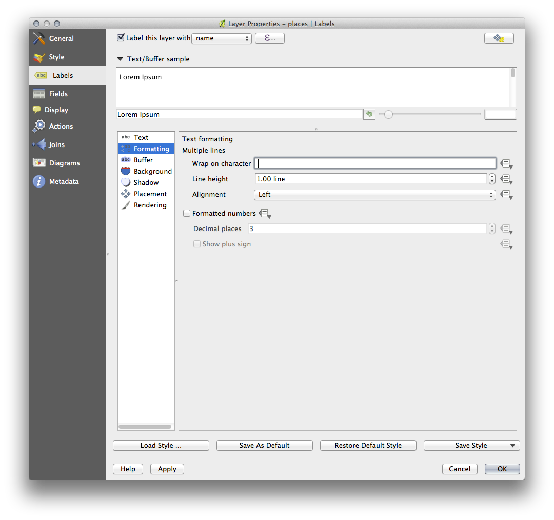
Enter a
spacein this field and click Apply to achieve the same effect. In our case, some of the place names are very long, resulting in names with multiple lines which is not very user friendly. You might find this setting to be more appropriate for your map.
21.7.3. Utilización de la configuración de definición de datos
Still in edit mode, set the
FONT_SIZEvalues to whatever you prefer. The example uses16for towns,14for suburbs,12for localities, and10for hamlets.Remember to save changes and exit edit mode
Return to the Text formatting options for the
placeslayer and selectFONT_SIZEin the Attribute field of the font size data defined override dropdown:
Sus resultados, si usó los valores antes mencionados, debería ser esto:
21.8. Results For Clasificación
21.8.1. Refinar la clasificación
Usa el nombre del método como en el primer ejercicio de la lección para deshacerse de los límites:
Los ajustes utilizados pueden no ser los mismos, pero con los valores Clases = 6 y Modo = Natural Breaks(Jenks) (y usando los mismos colores, por supuesto), el mapa se verá así:
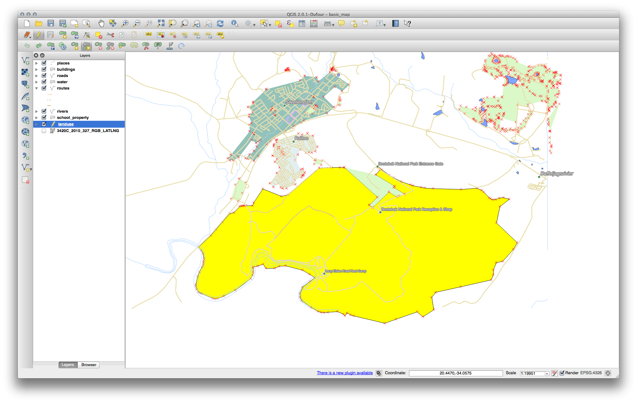
21.9. Results For Creando un nuevo conjunto de datos vector
21.9.1. Digitalizar
La simbología no importa, pero los resultados deberían verse más o menos como esto:
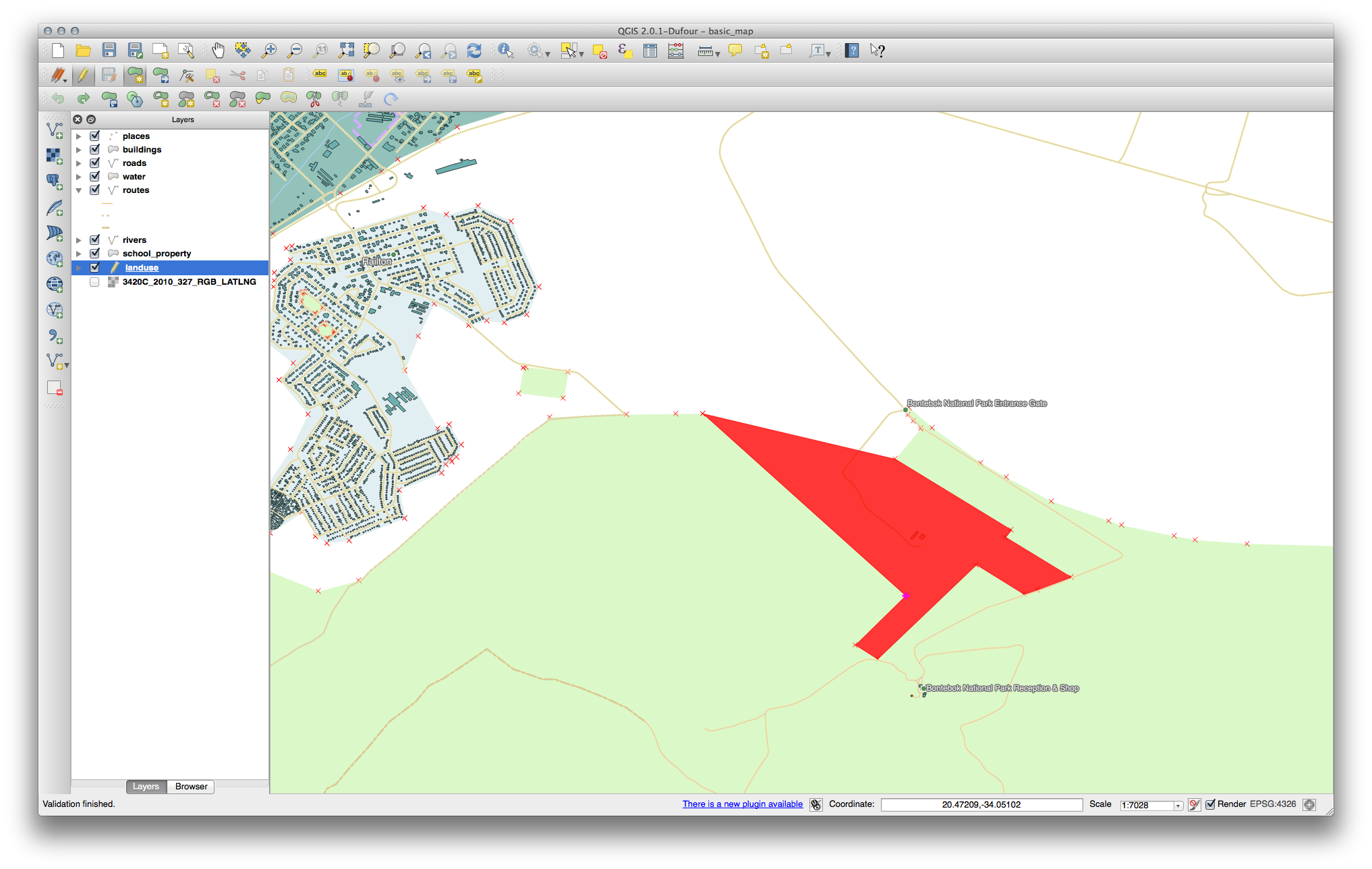
21.9.2. Topología: Herramienta de agregar anillo
La forma exacta no importa, pero debería estar recibiendo un agujero en medio de su rasgo, como la siguiente:

Deshacer su edición antes de continuar con el ejercicio con la siguiente herramienta.
21.9.3. Topología: Herramienta de agregar parte
Primero selecciona el Bontebok National Park:
Ahora agregar su nueva parte:
Deshacer su edición antes de continuar con el ejercicio con la siguiente herramienta.
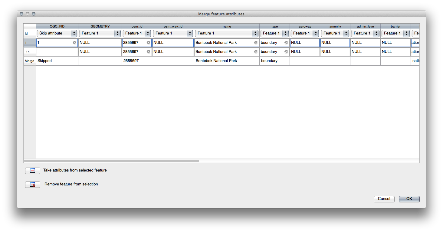
21.9.4. Unir objetos espaciales
Use la herramienta Merge Selected Features, para estar seguro, primero seleccione los poligonos que desee unir.
Use el rasgo con el OGC_FID de 1 como la fuente de sus atributos (clic en la entrada correspondiente de la ventana de dialogo, después clic en el botón Tomar los atributos del rasgo seleccionado):
Nota
- Si estas usando diferente conjunto de datos, es altamente probable que su
Polígono original OGC_FID no será 1. Solo tiene que elegir el rasgo que tiene un OGC_FID.
Nota
Usando la herramienta Unir atributos de los rasgos seleccionados mantendrá las distintas geometrías, pero les dará los mismo atributos.
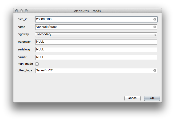
21.9.5. Formas
Para el TIPO, hay obviamente un cantidad límite de tipos que una carretera puede tener, si revisa la tabla de atributos de la capa, verá que están predefinidos.
Establecer el widget a Valor del mapa y clic Cargar datos de la capa.
Seleccionar Carreteras in el Etiqueta desplegable y autopista para ambos las opciones de Valor y Descripción:

Click OK three times.
Si usa la herramienta Identificación en una calle mientras esta activo el modo edición, la ventana de dialogo que deberías ver será como esto:
21.10. Results For Análisis Vector
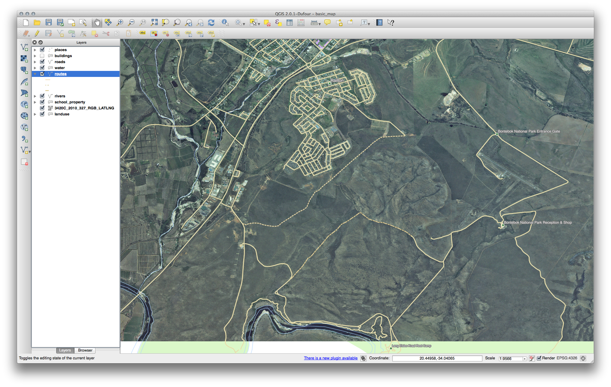
21.10.1. Distancia desde institutos
Su diálogo de buffer debería parecerse a esto:
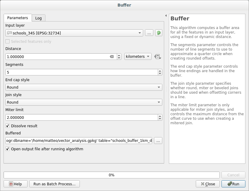
The Buffer distance is 1 kilometer.
The Segments to approximate value is set to 20. This is optional, but it’s recommended, because it makes the output buffers look smoother. Compare this:

A esto:

The first image shows the buffer with the Segments to approximate value set to 5 and the second shows the value set to 20. In our example, the difference is subtle, but you can see that the buffer’s edges are smoother with the higher value.
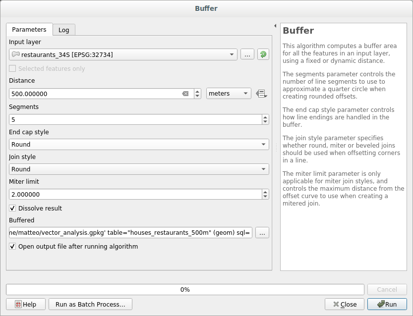
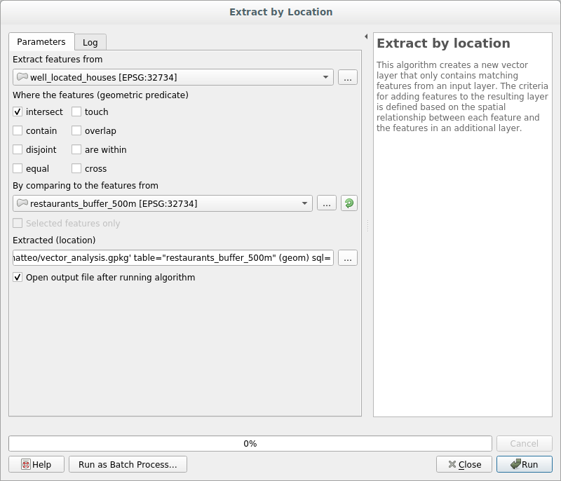
21.10.2. Distancia de restaurantes
To create the new houses_restaurants_500m layer, we go through a two step process:
Primero, crear un buffer de 500m alrededor de los restaurantes y agregar la capa al mapa:

Next, extract buildings within that buffer area:
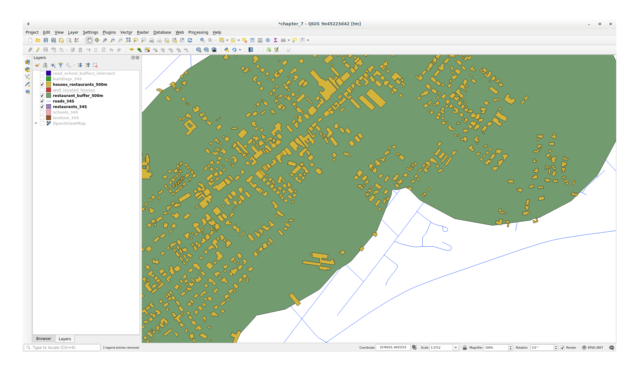
Su mapa debe mostrar solo aquellos edificios que estén a menos de 50m de la carretera, 1 km de la escuela y 500m de un restaurante:
21.11. Results For Network Analysis
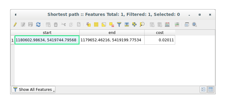
21.12. Fastest path
Open and fill the dialog as:

Make sure that the Path type to calculate is Fastest.
Click on Run and close the dialog.
Open now the attribute table of the output layer. The cost field contains the travel time between the two points (as fraction of hours):
21.13. Results For Análisis Raster


21.13.2. Calcular pendiente (menos de 2 y 5 grados)
Establezca su dialogo Calculadora Raster como esto:
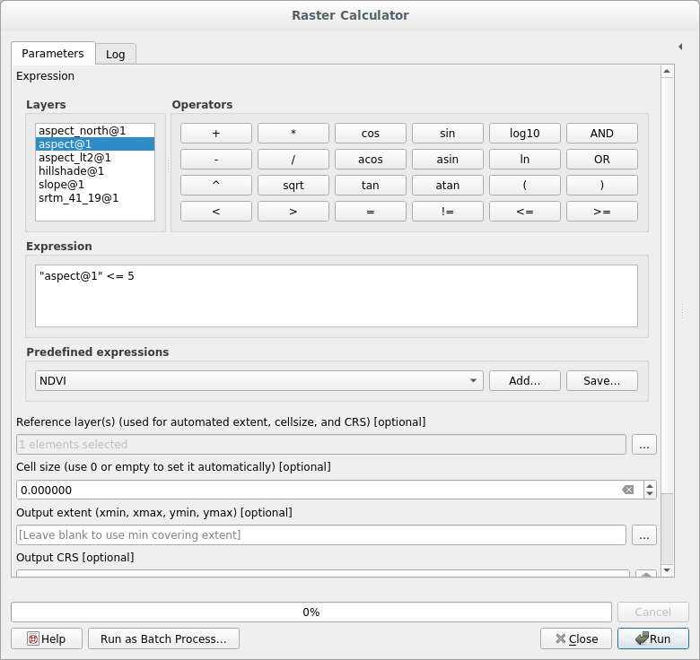
For the 5 degree version, replace the
2in the expression and file name with5.
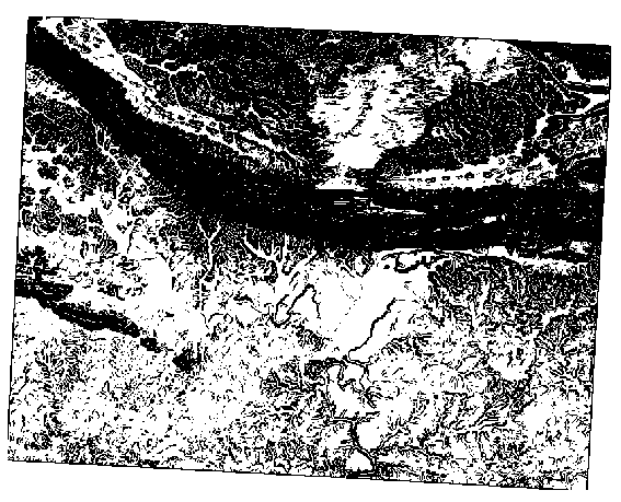
Sus resultados:
2 grados:

5 grados:
21.14. Results For Completando el Análisis
21.14.1. de Raster a Vector
Open the Query Builder by right-clicking on the all_terrain layer in the Layers panel, and selecting the tab.
Después construir la consulta "suitable" = 1.
Clic OK para filtrar todos los polígonos que no cumplan con esa condición.
Cuando vea el raster original, el área debe sobreponerse perfectamente:

You can save this layer by right-clicking on the all_terrain layer in the Layers panel and choosing Save As…, then continue as per the instructions.
21.14.2. Revisando los resultados
Podrá notar que algunos de los edificios en su capa nueva_solución han sido «cortados» por la herramienta Intersectar. Esto muestra que sólo parte del edificio -y por lo tanto solamente parte de la propiedad- se ubica en un terreno adecuado. Podemos entonces con seguridad eliminar esos edificios de nuestro Conjunto de datos.
21.14.3. Afinando el Análisis
Por el momento, su análisis deberá verse más o menos así:
Considera un área circular, con 100 metros a la redonda
Si es más grande que 100 metros de radio, entonces extraer 100 metros de su tamaño (en todas las direcciones) resultará en que una parte de el quede sobrante en el medio.

Por lo tanto, puede ejecutar un buffer interior de 100 metros en su capa vectorial existente terreno_apto. En el resultado de la aplicación de la función buffer, lo que sea que quede en la capa original representará áreas en donde hay terreno apto más allá de los 100.
Para demostrar:
Ir a para abrir el diálogo de Buffer(s).
Configúralo así:

Use la capa terreno_apto con 10 segmentos y una distancia de buffer de -100. (La distancia es automáticamente reconocida en metros debido a que su mapa está usando un SRC proyectado).
Guarda la capa resultante en datos_ejercicio/desarrollo_residencial/ como terreno_apto_continuos100m.shp.
Si es necesario, mueva la nueva capa encima de su capa original terreno_apto.
Sus resultados se verán más o menos así:

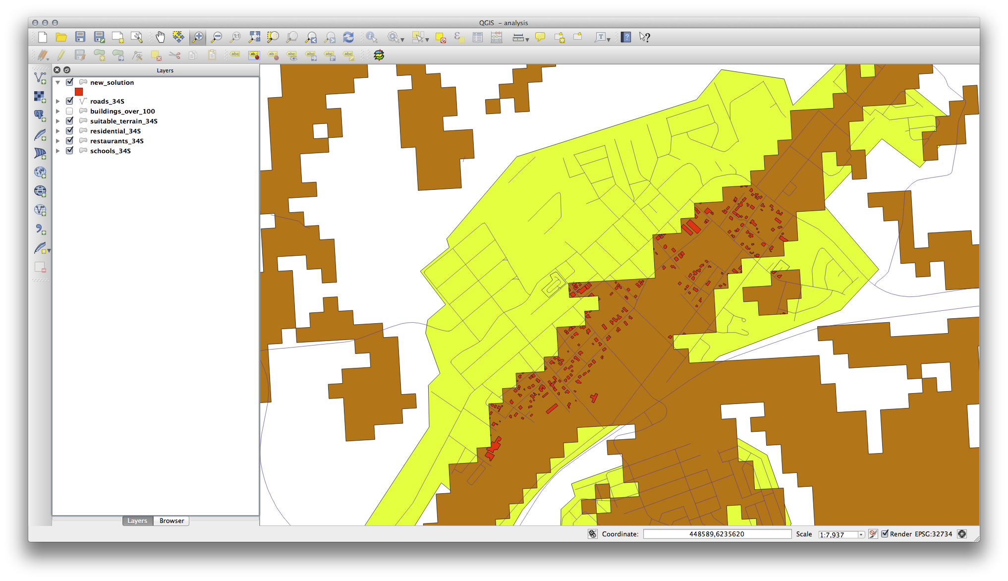
Ahora utilice la herramienta Selección por ubicación ().
Configurar de la siguiente manera:

Seleccione elementos en nueva_solución que intersecte elementos de terreno_apto_continuos100m.shp.
Este es el resultado:
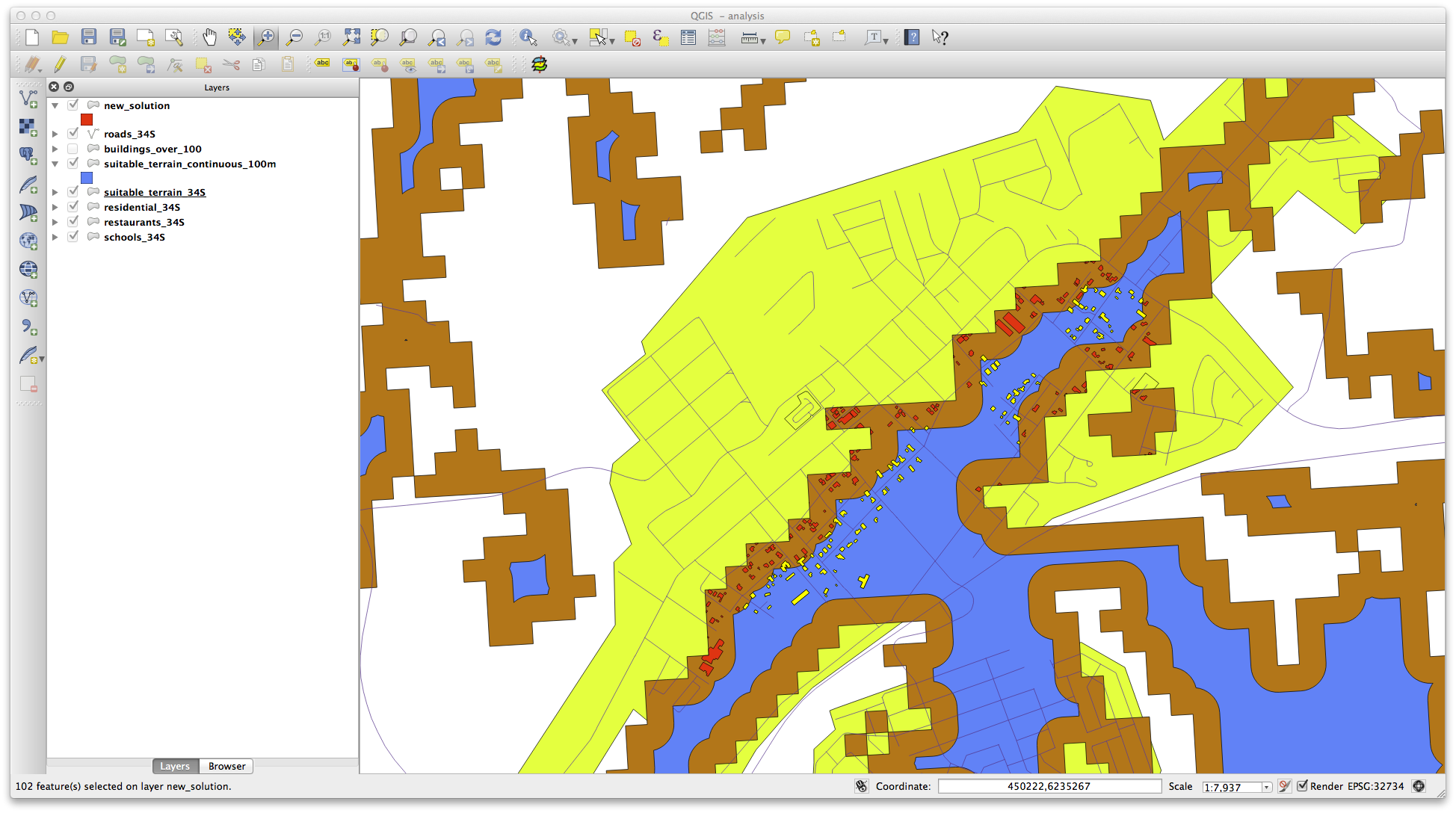
Los edificios en color amarillo están seleccionados. Aunque algunos de los edificios caen parcialmente afuera de la nueva capa terreno_apto_continuos100m.shp, caen bien dentro de la capa original terreno_apto y por lo tanto cumplen con todos nuestros requerimientos.
Guarde la selección en datos_ejercicio/desarrollo_residencial/ con el nombre respuesta_final.shp.
21.15. Results For WMS
21.15.1. |FA| Cargar otra Capa WMS
Su mapa debería verse así (puede que necesite re-ordenar las capas):

21.15.2. Agregando un Nuevo Servidor WMS
Utilice el mismo método que antes para agregar el nuevo servidor y la capa adecuada según como se encuentre alojada en el servidor:


Si realiza un acercamiento en el área Swellendam, notará que este conjunto de datos tiene una baja resolución.
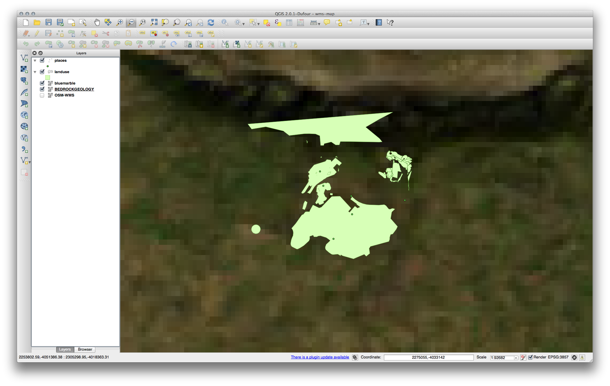
Por lo tanto, es mejor no usar este dato para el mapa actual. El dato de Blue Marble es más apropiado para las escalas nacionales y globales.
21.15.3. Agregando un Nuevo Servidor WMS
You may notice that many WMS servers are not always available. Sometimes this is temporary, sometimes it is permanent. An example of a WMS server that worked at the time of writing is the World Mineral Deposits WMS at http://apps1.gdr.nrcan.gc.ca/cgi-bin/worldmin_en-ca_ows. It does not require fees or have access constraints, and it is global. Therefore, it does satisfy the requirements. Keep in mind, however, that this is merely an example. There are many other WMS servers to choose from.
21.16. Results For GRASS Integration
21.16.1. Add Layers to Mapset
You can add layers (both vector and raster) into a GRASS Mapset by drag and drop
them in the Browser (see Follow Along: Load data using the QGIS Browser) or by using the v.in.gdal.qgis
for vector and r.in.gdal.qgis for raster layers.
21.16.2. Reclassify raster layer
To discover the maximum value of the raster run the r.info tool: in the console you will see that the maximum value is 1699.
You are now ready to write the rules. Open a text editor and add the following rules:
0 thru 1000 = 1
1000 thru 1400 = 2
1400 thru 1699 = 3
save the file as a my_rules.txt file and close the text editor.
Run the r.reclass tool, choose the g_dem layer and load the file containing the rules you just have saved.
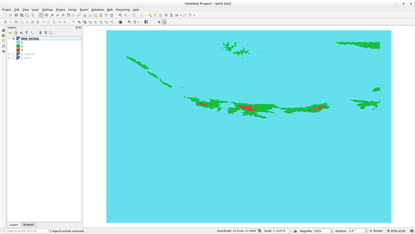
Click on Run and then on View Output. You can change the colors and the final result should look like the following picture:
21.17. Results For Conceptos de Bases de Datos
21.17.1. Propiedades de la Tabla de Direcciones
Para nuestra tabla de direcciones teórica, podríamos querer almacenar las siguientes propiedades:
House Number
Street Name
Suburb Name
City Name
Postcode
Country
Al crear la tabla para representar un objeto de dirección, crearemos columnas para representar cada una de estas propiedades y les estaríamos asignando nombres compatibles con SQL y posiblemente nombres cortos
house_number
street_name
suburb
city
postcode
country
21.17.2. Normalizando la Tabla de Personas
El mayor problema con la capa de gente es que hay solo un campo de dirección que contiene los datos de domicilio de las personas. Pensando en nuestra tabla teórica direccion anteriormente en esta lección, sabemos que una dirección esta compuesta por varias propiedades. Mediante el almacenamiento de todas estas propiedades en un solo campo, con esto haremos mucho mas difícil la actualización y la consulta de nuestros datos. Por lo tanto tenemos que dividir el campo de dirección en varias propiedades. Esto nos daría una tabla que tenga las siguiente estructura:
id |     name      | house_no |  street_name   |    city    |   phone_no
 --+---------------+----------+----------------+------------+-----------------
 1 | Tim Sutton    |     3    | Buirski Plein  | Swellendam | 071 123 123
 2 | Horst Duester |     4    | Avenue du Roix | Geneva     | 072 121 122
Nota
En la siguiente sección, aprenderemos acerca de relaciones de llave foránea, que podrán ser usados en este ejemplo para mejorar aún más la estructura de nuestra base de datos.
21.17.3. Además normalización de la tabla de Personas
Actualmente nuestra tabla de personas se ve así:
id |     name     | house_no | street_id |  phone_no
---+--------------+----------+-----------+-------------
 1 | Horst Duster |        4 |         1 | 072 121 122
La columna street_id representa una relacion “uno a muchos” entre el objeto personas y el objeto relacionado calle, que esta en la tabla de calles.
Una forma para normalizar aún más la tabla es dividir el nombre del campo en nombre y apellido:
id | first_name | last_name  | house_no | street_id |  phone_no
---+------------+------------+----------+-----------+------------
 1 |    Horst   |   Duster   |     4    |     1     | 072 121 122
Podemos crear también tablas independientes para nombre pueblo o ciudad y país, enlazándolos a nuestra tabla de personas a través de una relación de “uno a muchos”:
id | first_name | last_name | house_no | street_id | town_id | country_id
---+------------+-----------+----------+-----------+---------+------------
 1 |    Horst   |   Duster  |     4    |     1     |    2    |     1
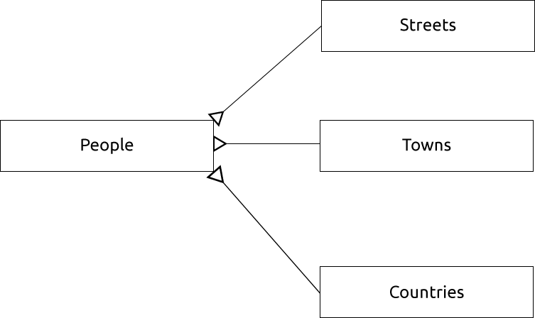
Un diagrama de ER para representar esto sería así:
21.17.4. Crear una tabla de Personas
El SQL necesario para crear la tabla correcta de personas es:
create table people (id serial not null primary key,
                     name varchar(50),
                     house_no int not null,
                     street_id int not null,
                     phone_no varchar null );
El esquema para la tabla (introduzca \d people) se ve así:
Table "public.people"

Column     |         Type          |                      Modifiers
-----------+-----------------------+-------------------------------------
id         | integer               | not null default
           |                       | nextval('people_id_seq'::regclass)
name       | character varying(50) |
house_no   | integer               | not null
street_id  | integer               | not null
phone_no   | character varying     |
Indexes:
  "people_pkey" PRIMARY KEY, btree (id)
Nota
Para fines de ilustración, hemos omitido a propósito la restricción del fkey.
21.17.5. El comando DROP
El motivo del comando DROP no funcionaría en este caso, porque la tabla personas tiene un restricción de llave foránea para la tabla calles. Esto significa que dropping (o eliminar) la tabla de calles dejaría a la tabla de personas con las referencias a calles de datos no existentes.
Nota
Es posible para “fuerza” la tabla de calles para ser eliminado mediante el uso del comando CASCADE, pero también se eliminaría la tabla de personas y alguna otra que tenga relación con la tabla calles. ¡Utilizar con precaución!
21.17.6. Insertar una nueva calle
El comando SQL, que debe usar se ve así (puede reemplazar el nombre de la calle con uno de su elección):
insert into streets (name) values ('Low Road');
21.17.7. Agregar una nueva persona con relación de llave foránea
Aquí esta la sentencia SQL correcta:
insert into streets (name) values('Main Road');
insert into people (name,house_no, street_id, phone_no)
  values ('Joe Smith',55,2,'072 882 33 21');
Si se fija en la tabla de calles nuevamente (utilizando una sentencia select como antes), vera que el id de la entidad Carretera Principal es 2.
Eso es por qué podríamos solo introducir el numero 2 arriba. Aunque no estemos viendo Carretera principal escrito completamente en la entrada de arriba, la base de datos podrá estar asociada a street_id con el valor de 2.
Nota
Si ya ha añadido un nuevo objeto street, puede encontrarse con que el nuevo Main Road tiene un ID de 3 y no de 2.
21.17.8. Regresar Nombre de calles
Aquí esta la sentencia SQL correcta que debe usar:
select count(people.name), streets.name
from people, streets
where people.street_id=streets.id
group by streets.name;
Resultado:
count |    name
------+-------------
    1 | Low Street
    2 | High street
    1 | Main Road
(3 rows)
Nota
Se dará cuenta de que hemos prefijado nombres de campo con nombres de tablas (por ejemplo people.name y streets.name). Esto se debe hacer cada vez que el nombre de campo sea ambiguo (es decir no es único en todas las tablas de la base de datos)
21.18. Results For Consultas Espaciales
21.18.1. Las unidades usadas en Consultas Espaciales
Las unidades usadas para el ejemplo de consulta son grados, porque el SRC que la capa esta usando es WGS84. Este es un SRC Geografico, que significa que las unidades están en grados. Un proyecto SRC, como la proyección UTM que esta en metros.
Recuerde que cuando escriba la consulta, necesita saber en que unidades esta el SRC de la capa. Esto te permitirá escribir una consulta que regrese los resultados que tu esperas.
21.18.2. Creando un índice espacial
CREATE INDEX cities_geo_idx
  ON cities
  USING gist (the_geom);
21.19. Results For Construcion de geometría
21.19.1. Creando linestrings
alter table streets add column the_geom geometry;
alter table streets add constraint streets_geom_point_chk check
     (st_geometrytype(the_geom) = 'ST_LineString'::text OR the_geom IS NULL);
insert into geometry_columns values ('','public','streets','the_geom',2,4326,
     'LINESTRING');
create index streets_geo_idx
  on streets
  using gist
  (the_geom);
21.19.2. «Enlazando tablas»
delete from people;
alter table people add column city_id int not null references cities(id);
(capturar ciudades en QGIS)
insert into people (name,house_no, street_id, phone_no, city_id, the_geom)
   values ('Faulty Towers',
           34,
           3,
           '072 812 31 28',
           1,
           'SRID=4326;POINT(33 33)');

insert into people (name,house_no, street_id, phone_no, city_id, the_geom)
   values ('IP Knightly',
           32,
           1,
           '071 812 31 28',
           1,F
           'SRID=4326;POINT(32 -34)');

insert into people (name,house_no, street_id, phone_no, city_id, the_geom)
   values ('Rusty Bedsprings',
           39,
           1,
           '071 822 31 28',
           1,
           'SRID=4326;POINT(34 -34)');
Si recibe el siguiente mensaje de error:
ERROR:  insert or update on table "people" violates foreign key constraint
        "people_city_id_fkey"
DETAIL: Key (city_id)=(1) is not present in table "cities".
entonces significa que mientras experimentaba con la creación de polígonos para la tabla de ciudades, debe haber eliminado algunos de ellos y empezar de nuevo. Vea las entradas de su tabla de ciudades y use cualquier id que exista.
21.20. Results For Modelo de características simples
21.20.1. Llenar tablas
create table cities (id serial not null primary key,
                     name varchar(50),
                     the_geom geometry not null);
 alter table cities
 add constraint cities_geom_point_chk
 check (st_geometrytype(the_geom) = 'ST_Polygon'::text );
21.20.2. Llenar la tabla Geometria_Columnas
insert into geometry_columns values
      ('','public','cities','the_geom',2,4326,'POLYGON');
21.20.3. Agregar geometría
select people.name,
       streets.name as street_name,
       st_astext(people.the_geom) as geometry
from   streets, people
where  people.street_id=streets.id;
Resultado:
     name     | street_name |   geometry
--------------+-------------+---------------
 Roger Jones  | High street |
 Sally Norman | High street |
 Jane Smith   | Main Road   |
 Joe Bloggs   | Low Street  |
 Fault Towers | Main Road   | POINT(33 -33)
(5 rows)
Como puede ver, nuestra limitación permite agregar nulos en la base de datos.