7.2. Lesson: Análisis Vectorial

También se puede proceder al análisis de datos vectoriales para saber cómo los distintos elementos interactúan entre sí en el espacio. Hay muchas funciones relacionadas con el análisis en SIG, así que no nos detendremos en todas ellas. En su lugar, plantearemos una pregunta e intentaremos resolverla utilizando las herramientas proporcionadas por QGIS.

El objetivo de esta lección: Plantear una pregunta y contestarla utilizando las herramientas de análisis.

7.2.1. El proceso SIG

Antes de comenzar, sería de utilidad conocer de manera general los pasos que podemos seguir para resolver cualquier problema SIG. Lo que debemos hacer es lo siguiente:

1. Plantear el problema

2. Obtener los datos

3. Analizar el problema

4. Presentar los resultados

7.2.2. The Problem

Comencemos este procedimiento eligiendo un problema que se deba resolver. Por ejemplo, imaginemos que eres un agente inmobiliario que está buscando un inmueble en Swellendam para clientes con el siguiente perfil:

1. It needs to be in Swellendam

2. It must be within reasonable driving distance of a school (say 1km)

3. It must be more than 100m squared in size

4. Closer than 50m to a main road

5. Closer than 500m to a restaurant

7.2.3. The Data

Para resolver todas estas preguntas, vamos a necesitar los siguientes datos:

1. The residential properties (buildings) in the area

2. The roads in and around the town

3. The location of schools and restaurants

4. The size of buildings

All of this data is available through OSM and you should find that the dataset you have been using throughout this manual can also be used for this lesson.

If you want to download data from another area jump to Introduction Chapter section to read how to do it.

Nota

Aunque hay coherencia en los campos de datos que encontramos en las descargas de OSM, pueden variar en su cobertura y detalle. Si ves, por ejemplo, que la región que has elegido no contiene información sobre restaurantes, quizás necesitas elegir otra región.

7.2.4. Follow Along: Start a Project and get the Data

We first need to load the data to work with.

1. Start a new QGIS project

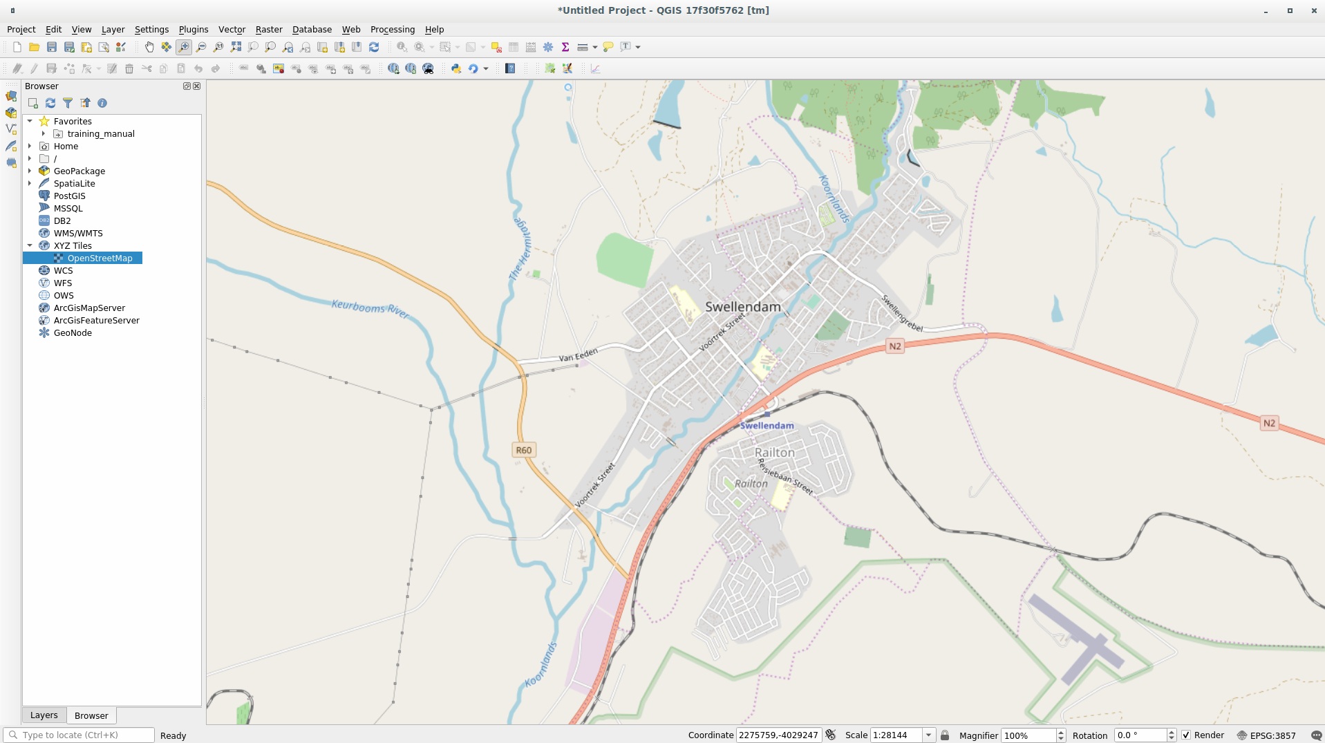
2. If you want you can add a background map. Open the Browser and load the OSM background map from the XYZ Tiles menu.

   

3. In the training_data.gpkg Geopackage database load all the files we will use in this chapter:

   1. landuse

   2. buildings

   3. roads

   4. restaurants

   5. schools

4. Zoom to the layer extent to see Swellendam, South Africa

Before proceeding we should filter the roads layer in order to have only some specific road types to work with.

Some of the roads in OSM dataset are listed as unclassified, tracks, path and footway. We want to exclude these from our dataset and focus on the other road types, more suitable for this exercise.

Moreover, OSM data might not be updated everywhere and we will also exclude NULL values.

1. Right click on the roads layer and choose Filter….

2. In the dialog that pops up we can filter these features with the following expression:

   "highway" NOT IN ('footway','path','unclassified','track') OR "highway" != NULL
   

   The concatenation of the two operators NOT and IN means to exclude all the unwanted features that have these attributes in the highway field.

   != NULL combined with the OR operator is excluding roads with no values in the highway field.

   You will note the icon next to the roads layer that helps you remember that this layer has a filter activated and not all the features are available in the project.

The map with all the data should look like the following one:

7.2.5. Try Yourself Convertir el SRC de una Capa

Because we are going to be measuring distances within our layers, we need to change the layers” CRS. To do this, we need to select each layer in turn, save the layer to a new one with our new projection, then import that new layer into our map.

You have many different options, e.g. you can export each layer as a new Shapefile, you can append the layers to an existing GeoPackage file or you can create another GeoPackage file and fill it with the new reprojected layers. We will show the last option so the training_data.gpkg will remain clean. But feel free to choose the best workflow for yourself.

Nota

En este ejemplo, vamos a usar el SRC WGS 84 / UTM zone 34S, pero puedes utilizar un SRC UTM que sea más apropiado para tu región.

1. Right click the roads layer in the Layers panel;

2. Click Export –> Save Features As…;

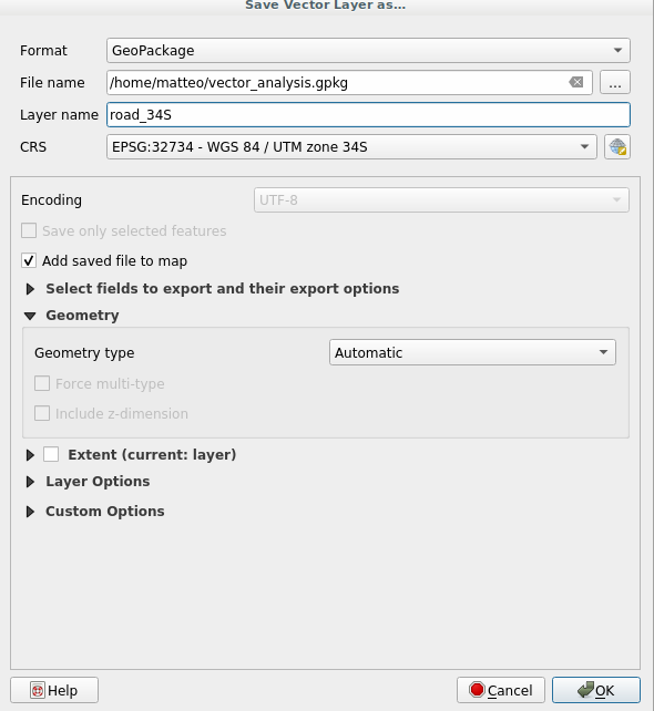
3. In the Save Vector Layer As dialog choose GeoPackage as Format;

4. Click on … of File name parameter and name the new GeoPackage as vector_analysis;

5. Change the Layer name as roads_34S;

6. Change the CRS parameter to WGS 84 / UTM zone 34S;

7. Finally click on OK:

   

   This will create the new GeoPackage database and fill it with the roads_34S layer.

8. Repeat this process for each layer, creating a new layer in the vector_analysis.gpkg GeoPackage file with _34S appended to the original name and removing each of the old layers from the project.

   Nota

   When you choose to save a layer to an existing GeoPackage, QGIS will append that layer in the GeoPackage.

9. Una vez que hayas completado el proceso para cada capa, haz clic derecho sobre cualquiera de las capas y clic en Zum a la extensión de la capa para enfocar el mapa a la zona de interés.

Ahora que hemos convertido los datos OSM a una proyección UTM, podemos empezar nuestros cálculos.

7.2.6. Follow Along: Analizando el Problema: Distancias Desde Colegios y Carreteras.

QGIS te permite calcular distancias desde cualquier objeto vectorial.

1. Make sure that only the roads_34S and buildings_34S layers are visible, to simplify the map while you’re working

2. Click on the Processing ‣ Toolbox to open the analytical core of QGIS. Basically: all algorithms (for vector and raster) analysis are available within this toolbox.

3. We start by calculating the area around the roads_34S by using the Buffer algorithm. You can find it expanding the Vector Geometry group.

   

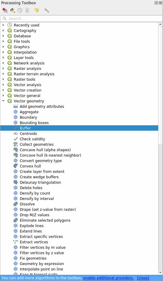
   Or you can type buffer in the search menu in the upper part of the toolbox: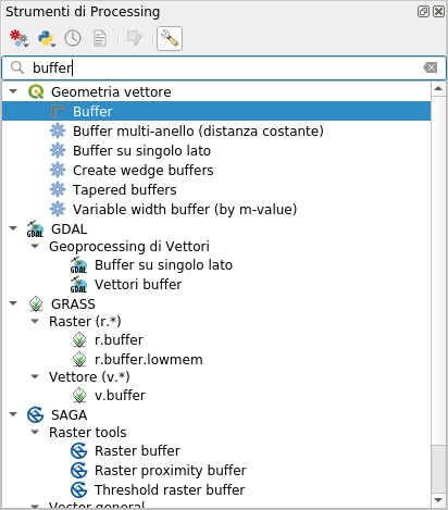

   

4. Double click on it to open the algorithm dialog

5. Set it up like this

   

6. The default Distance is in meters because our input dataset is in a Projected Coordinate System that uses meter as its basic measurement unit. You can use the combo box to choose other projected units like kilometers, yards, etc.

   Nota

   If you are trying to make a buffer on a layer with a Geographical Coordinate System, Processing will warn you and suggest to reproject the layer to a metric Coordinate System.

7. By default Processing creates temporary layers and adds them to the Layers panel. You can also append the result to the GeoPackage database by:

   1. clicking on the … button and choose Save to GeoPackage…

   2. naming the new layer roads_buffer_50m

   3. and saving it in the vector_analysis.gpkg file

   

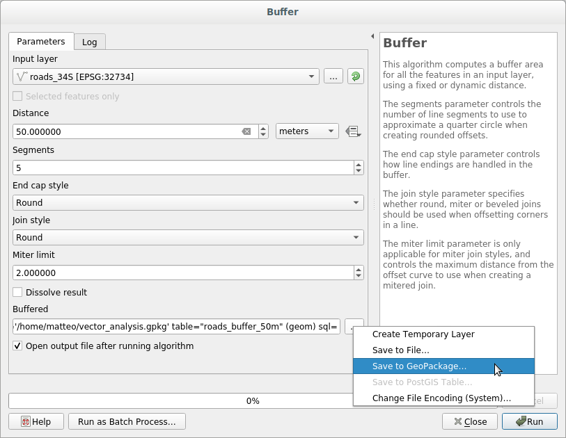
8. Click on Run and then close the Buffer dialog.

Ahora tu mapa se parece un poco a esto:

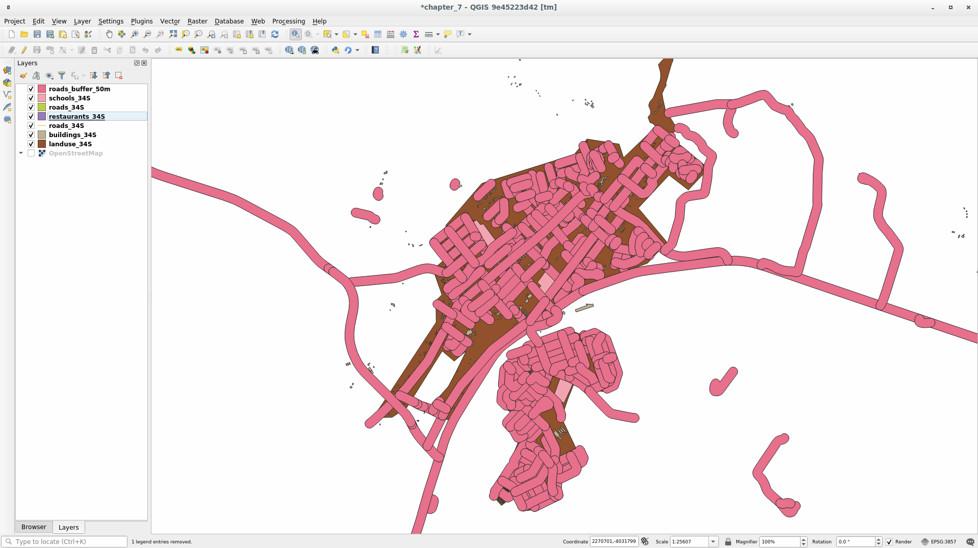
If your new layer is at the top of the Layers list, it will probably obscure much of your map, but this gives you all the areas in your region which are within 50m of a road.

However, you’ll notice that there are distinct areas within your buffer, which correspond to all the individual roads. To get rid of this problem:

1. Uncheck the roads_buffer_50m layer and re-create the buffer using the settings shown here:

   

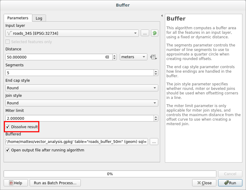
   Note that we’re now checking the Dissolve result box

2. Save the output as roads_buffer_50m_dissolved

3. Click Run and close the Buffer dialog again

Once you’ve added the layer to the Layers panel, it will look like this:

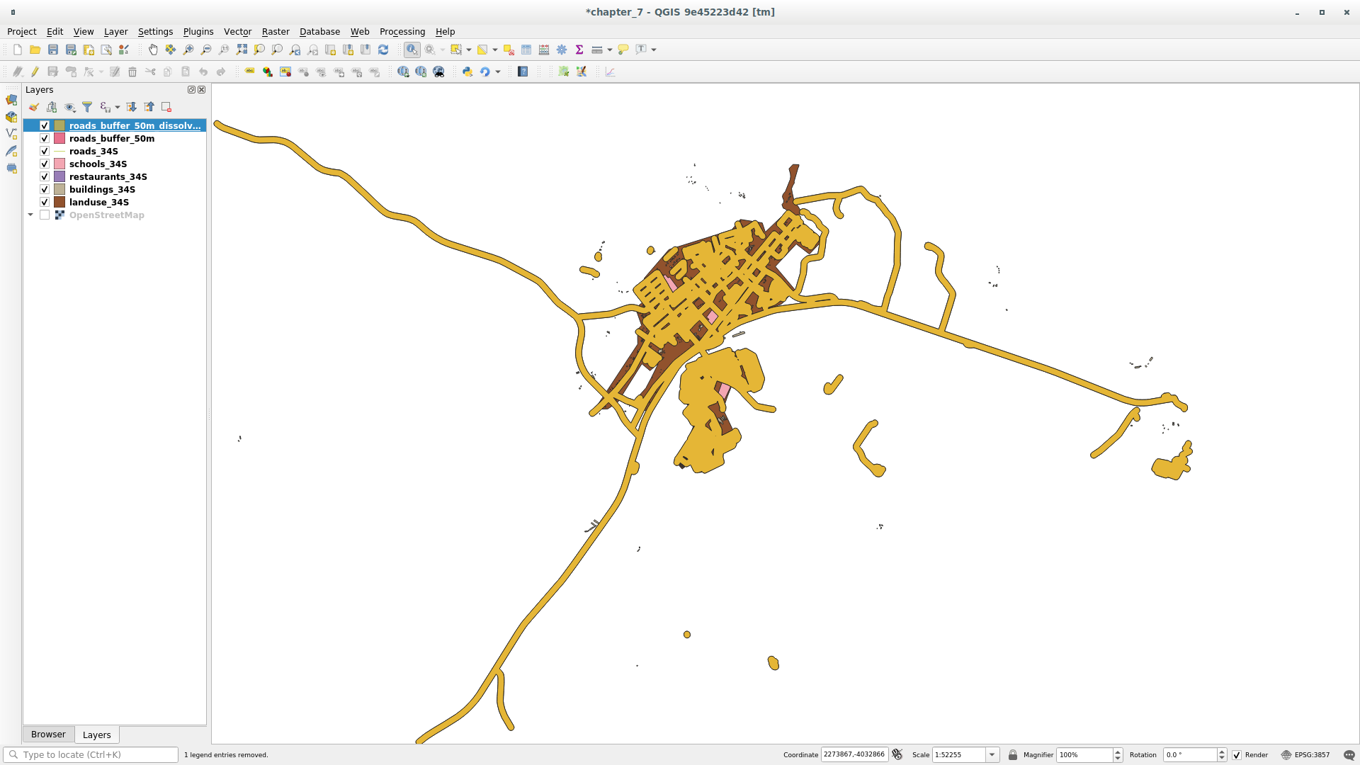
Ahora no hay subdivisiones innecesarias.

Nota

The Short Help on the right side of the dialog explains how the algorithm works. If you need more information, just click on the Help button in the bottom part to open a more detailed guide of the algorithm.

7.2.7. Try Yourself Distancia desde colegios.

Usa el mismo enfoque que anteriormente y crea un buffer para tus colegios.

It needs to be 1 km in radius. Save the new layer in the vector_analysis.gpkg file as schools_buffer_1km_dissolved.

Comprueba tus resultados

7.2.8. Follow Along: Areas que se solapan.

Now we have areas where the road is 50 meters away and there’s a school within 1 km (direct line, not by road). But obviously, we only want the areas where both of these criteria are satisfied. To do that, we’ll need to use the Intersect tool. You can find it in Vector Overlay group within Processing ‣ Toolbox.

1. Configúralo así:

   

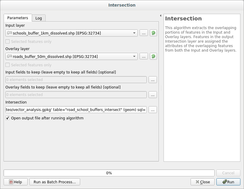
   • The input layers are the two buffers

   • The saving location is, once again, the vector_analysis.gpkg GeoPackage

   • And the output layer name is road_school_buffers_intersect

2. Click Run.

   En la imagen inferior, las áreas en azul muestran donde ambos criterios de distancia coinciden

   

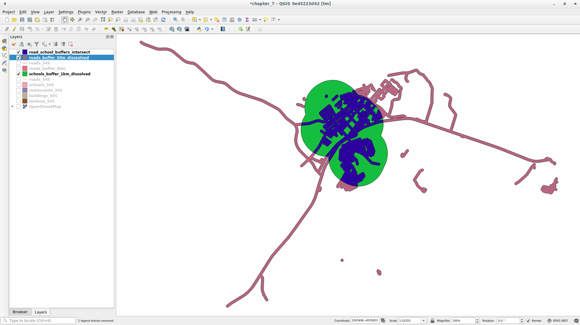
3. Usted puede borrar las dos capas buffer y solo mantener la que muestra la superposición, dado que eso era lo que queriamos conocer en primer lugar:

   

7.2.9. Follow Along: Extract the Buildings

Now you’ve got the area that the buildings must overlap. Next, you want to extract the buildings in that area.

1. Look for the menu entry Vector Selection ‣ Extract by location within Processing ‣ Toolbox

2. Set up the algorithm dialog like in the following picture

   

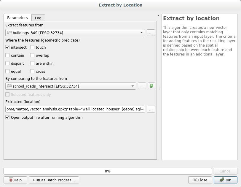
3. Click Run and then close the dialog

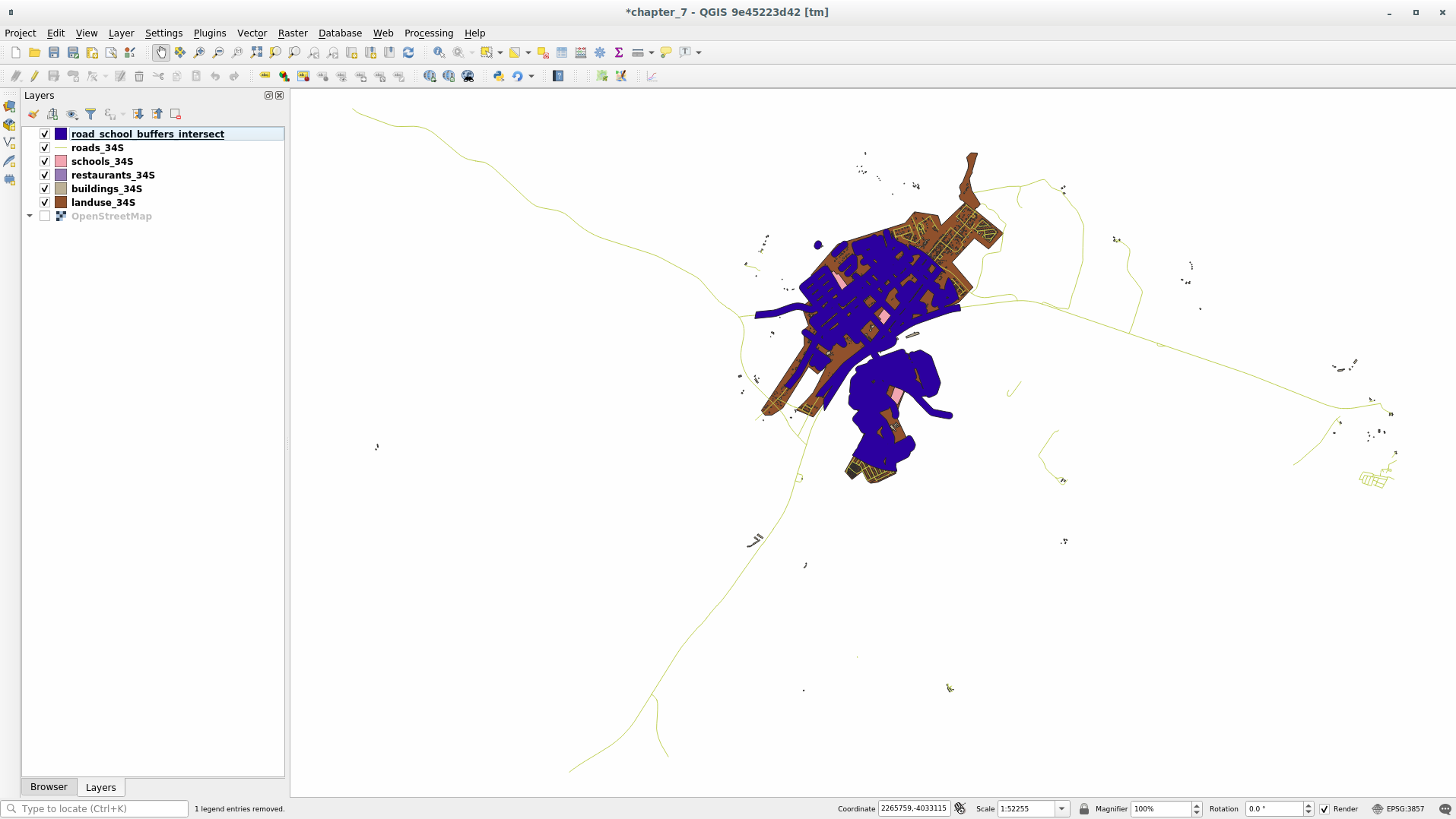
4. You’ll probably find that not much seems to have changed. If so, move the well_located_houses layer to the top of the layers list, then zoom in.

   

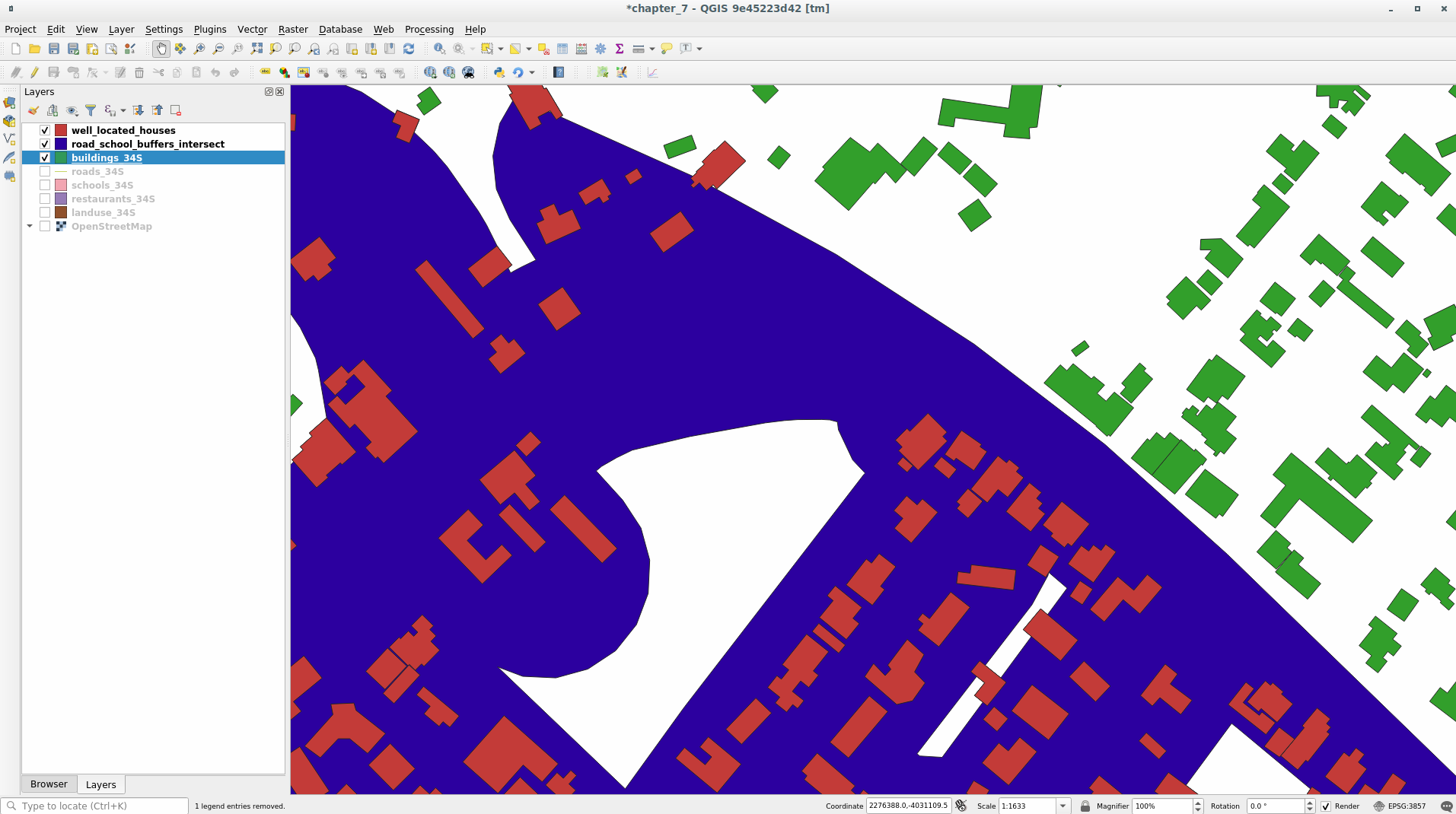
   The red buildings are those which match our criteria, while the buildings in green are those which do not.

5. Now you have two separated layers and can remove buildings_34S from layer list.

7.2.10. Try Yourself Filtrado adicional de nuestros Edificios

Ahora tenemos una capa que nos muestra los edificios en un radio de 1km de una escuela y a menos de 50m de una carretera. Ahora tenemos que reducir la selección para que sólo nos muestre los edificios que están a menos de 500 metros de un restaurante.

Using the processes described above, create a new layer called houses_restaurants_500m which further filters your well_located_houses layer to show only those which are within 500m of a restaurant.

:ref:` Comprueba tus resultados <vector-analysis-basic-2>`

7.2.11. Follow Along: Seleccione las Construcciones de Tamaño Adecuado

To see which buildings are of the correct size (more than 100 square meters), we first need to calculate their size.

1. Select the houses_restaurants_500m layer and open the Field Calculator by clicking on the button in the main toolbar or within the attribute table

2. Set it up like this

   

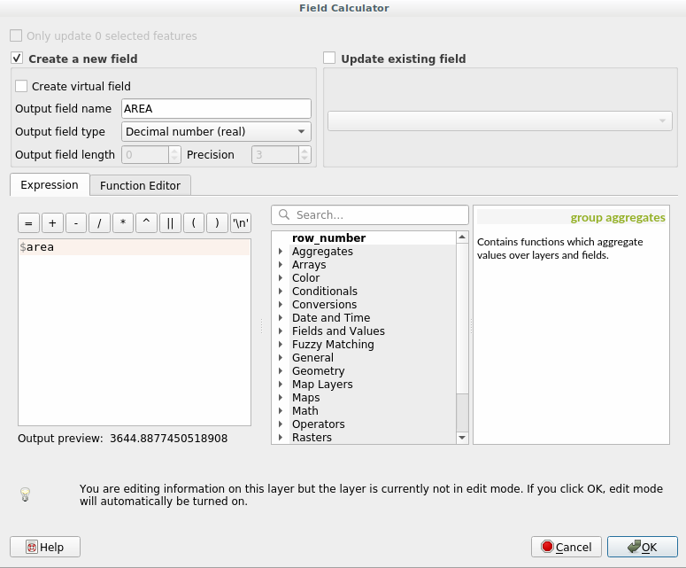
   We are creating the new field AREA that will contain the area of each building square meters.

3. Click OK. The AREA field has been added at the end of the attribute table.

4. Haga clic en el botón del modo de edición de nuevo para finalizar la edición y guarde los cambios cuando se le pida.

5. Build a query as earlier in this lesson

   

6. Haz clic en OK.

Your map should now only show you those buildings which match our starting criteria and which are more than 100m squared in size.

7.2.12. Try Yourself

Save your solution as a new layer, using the approach you learned above for doing so. The file should be saved within the same GeoPackage database, with the name solution.

7.2.13. In Conclusion

Usando la estrategia de resolución de problemas SIG junto con las herramientas de análisis vectorial de QGIS, has sido capaz de resolver un problema con múltiples criterios rápida y fácilmente.

7.2.14. What’s Next?

En la siguiente lección veremos como calcular la distancia mas corta de un punto a otro de una carretera.